Execution Timing, Jitter, and Derivative Filtering in High-Loop-Count PID Platforms

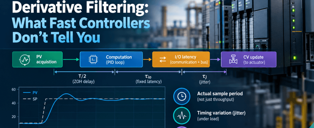
A controller that executes 1,000 PID loops in under 2 ms tells you something about throughput, but nothing about what each loop experiences. Loop quality depends on the sample period actually seen by each loop, the variation in that period, and the filter placed on the derivative term. This article derives how these three jointly erode phase margin and inflate noise on the manipulated variable, so you can decide whether a fast platform delivers what the spec sheet implies, or whether your loops still need the same scrutiny of scan timing as on a slow one.

Assumptions throughout: linear time-invariant plant approximated as first-order-plus-deadtime (FOPDT), uniform sampling at period T unless stated, zero-order-hold (ZOH) output, and SI units (seconds, rad/s).

Why execution rate is a design variable, not a spec line

A throughput figure such as “N loops per 2 ms” describes aggregate compute. It does not state:

• the period at which each loop is scheduled (a loop in a 100 ms task does not benefit from a fast CPU);
• the deterministic latency between the PV sample instant and the CV write instant;
• the jitter of that latency under load (communications, HMI, diagnostics, other tasks).

From the loop’s perspective, the computation-plus-I/O path is a delay. Sampling plus ZOH adds roughly T/2 of effective delay, plus any fixed input-to-output latency, plus jitter. All of it subtracts directly from phase margin at the crossover frequency. Execution rate is therefore a design parameter that sits alongside Kc, Ti and Td, and should be chosen against the process time constants and the desired closed-loop bandwidth.

Discrete PID structure, velocity vs positional form, and anti-windup interaction

Start from the continuous parallel-form PID with first-order derivative filter:

$K_c$ = proportional gain (CV units per PV unit), $T_i$ = integral time (s), $T_d$ = derivative time (s), $N$ = derivative filter factor (dimensionless, typically 5 to 20), $E = SP – PV$.

Discretize with backward differences for the integral and filtered derivative $\left(s → \frac{1 – z⁻¹}{T}\right)$. The positional form is:

The discrete filter pole can be written as $a=T_f/(T_f+T)$, where $T_f=T_d/N$. As $T$ becomes small relative to $T_f$, $a$ approaches 1, corresponding to a pole close to one in the discrete-time recursion. When $T=T_f$, $a=1/2$. The value $a=1/(1+N)$ occurs when $T=T_d$. Because the discrete coefficients depend on the sampling period, recalculate them whenever $T$ changes and verify the resulting closed-loop response. This does not automatically require changing the continuous-time tuning parameters $K_c$, $T_i$, or $T_d$.

Velocity form. Take the difference $u(k) – u(k-1)$ of the positional form. The integral sum collapses to a single term:

Key step: the $\Sigma e(j)$ term differences to $e(k)$, so no explicit integrator state is stored. The controller output is the accumulated increment.

Anti-windup interaction. In velocity form, windup is limited by clamping $u(k)$ to $\left[u_{min}, u_{max}\right]$ after accumulation, which is a form of integrator clamping because the output itself is the integrator. This is simple and bumpless on manual/auto transfer, but it ties the clamp to the actuator range only. With positional form you may choose conditional integration or back-calculation with tracking time $T_t$ (commonly between $\sqrt{T_i·T_d}$ and $T_i$). Back-calculation depends on $T_t$, which is an additional tuning dependence; velocity-form clamping has none but cannot account for downstream limits (e.g., a split-range or a rate-limited valve) unless the clamp is fed from the actual actuator position. Note that the proportional-on-error kick, SP weighting, and the choice of derivative on PV rather than error must be consistent across forms.

Sample period, zero-order-hold delay, and the phase lag it adds

A $ZOH$ of period $T$ has transfer function $\frac{1 – e^{-sT}}{s}$. At frequencies well below the sampling rate, it approximates a pure delay of $\frac{T}{2}$:

Where $sinc(x) = \frac{sin(x)}{x}$. The phase is exactly $-\frac{\omega T}{2}$. At the gain crossover frequency $\omega_c$, the added phase lag is:

Adding sample-and-hold delay and a fixed computational (or I/O) latency $\tau_{io}$, the total effective delay is:

where $\tau_j$ is the jitter bound (next section). Phase margin of the loop, relative to a design with no timing effects, falls as:

$PM_0$ = phase margin of the continuous design. This is first-order: valid when $\omega_c·T$ is well below $\pi$ (rule of thumb: $\omega_c·T < 0.5$). Beyond that the $sinc$ magnitude droop and aliasing matter, and the delay approximation understates degradation.

Derivative filtering: N-factor, noise amplification, and the bandwidth trade-off

The derivative term with first-order filter is:

Derivation of the high-frequency limit: as $s → \infin$, the “1” in the denominator is negligible against $s\frac{T_d}{N}$, so

In the form $K_d·s/(1 + s·\frac{T_d}{N})$ with $K_d = K_c·T_d$ (the derivative gain in CV·s per PV unit), the limit is $K_d·N/T_d = K_c·N$. This is the high-frequency gain of the controller from measurement noise to CV. For PV noise of standard deviation $\sigma_n$, CV noise scales roughly as $K_c·N·\sigma_n$ (bounded by the sampling Nyquist band). Doubling $N$ approximately doubles the high-frequency noise gain.

Trade-off: the filter corner is at $\omega = N/T_d$. Raising $N$ pushes the corner up, giving the derivative more phase lead near $\omega_c$, but amplifies noise and actuator wear. A low $N$ limits noise but reduces useful lead, and the filter itself adds lag at $\omega_c$ of $atan(\omega_c·T_d/N)$. With $T$-dependent discretization, there is a further constraint: $T_f = T_d/N$ should be at least about $2T$, otherwise the filter is effectively bypassed and the derivative acts on a single sample difference.

Execution jitter and its effect on loop stability margins

Let $\tau_{io}$ be the nominal latency between PV acquisition and CV update. Define $\tau_j$ as the maximum deviation of the actual input-to-output latency from its nominal value:$$\tau_j=\max_k\left|(t_{o,k}-t_{s,k})-\tau_{io}\right|$$

where $t_{s,k}$ and $t_{o,k}$ are the actual PV-sampling and CV-update times for scan $k$. If the sampling and output-update instants deviate from their nominal schedules by at most $\delta_i$ and $\delta_o$, respectively, a conservative bound is:

Where $\delta_i$ is the maximum absolute input sampling-time deviation, in seconds, and $\delta_o$ is the maximum absolute output update-time deviation, in seconds. PM degradation from jitter, to first order:

Jitter also perturbs the discrete integral and derivative: the integral accumulates $K_c·(T/Ti)·e(k)$ assuming nominal $T$, so a late sample under-integrates and an early one over-integrates, while the derivative difference $e(k) – e(k-1)$ divided by the nominal $T$ misreports slope by the factor $T_{actual}/T$. Derivative noise from jitter is proportional to the PV rate of change, so it matters most during setpoint moves and disturbances rather than steady state. If your platform exposes the true elapsed time per scan, compute $T_{actual}$ and use it in the algorithm.

Worked example: T = 10 ms vs T = 100 ms on an FOPDT process

Process: $G(s) = K_p · e^{-θs} / (τs + 1)$, with $K_p = 1$, $\tau = 20 s$, $\theta = 2 s$.

Tune a PI controller by a lambda/IMC rule with closed-loop time constant $\lambda = 2θ$. Here choose λ = 4 s:

Approximate crossover: $\omega_c \approx 1/(\lambda+\theta)=1/6\approx0.167\ \text{rad/s}$. Since $T_i=\tau=20\ \text{s}$, the PI controller and first-order process contribute a combined phase lag of $90^\circ$ at crossover. The process dead time contributes an additional lag of $\theta\omega_c=2/6=0.333\ \text{rad}=19.1^\circ$. Therefore, the continuous-time phase margin before sampling, I/O latency, and jitter is: $PM_0​≈180\degree−90\degree−19.1\degree=70.9\degree$.

Case A, $\bold{T = 10 \enskip ms}$, $\bold{\tau_j = 1 \enskip ms}$, $\bold{\tau_{io} = 2 \enskip ms}$:

Negligible. The timing contributes essentially nothing relative to $θ = 2 s$.

Case A, $\bold{\tau_j = 20 \enskip ms}$, $\bold{\tau_j = 20 \enskip ms}$, $\bold{\tau_{io} = 10 \hspace{0.5em} ms}$:

Also small. Conclusion for this slow loop: $T = 100 ms$ is adequate, and the 10 ms platform buys almost nothing. A useful screen: sample at $T ≤ θ/10$ or $T ≤ (λ+θ)/20$ here, either gives roughly 100 to 300 ms.

Contrast: a fast loop. Pressure or flow loop with $\theta = 0.2 s, \enskip \tau = 1 s, \enskip \lambda = 0.4 s$ gives $\omega_c ≈ 1/0.6 \approx 1.67 rad/s$. With $T = 100 ms$, jitter 20 ms, $\tau_{io} = 10 ms$: $\tau_{eff} = 0.08 s, \enskip \Delta PM = 1.67 · 0.08 = 0.133 rad = 7.6\degree$. With $T = 10 ms$ ($\tau_{eff} = 0.008 s$): 0.8°. Here the scan period matters: a 7.6° loss from 70.9° is tolerable but eats into the margin intended for model error. If $\tau$ shrinks further, the approximation $\omega_cT < 0.5$ and the loss grows linearly.

Derivative noise at the same two rates. For a PID with $K_c = 3.33, N = 10$, PV noise $\sigma_n = 0.2 \%$ of span: high-frequency CV noise $\approx K_c·N·\sigma_n = 3.33 · 10 · 0.2\% = 6.7\%$ of span, at either $T$, bounded by Nyquist. Faster sampling does not reduce this; it increases the bandwidth over which noise reaches the valve. Reduce $N$ or filter the PV first.

Tuning rules for a fast-scan platform and commissioning checks

• Choose $T$ from the process: $T \approx \theta/10$ to $θ/5$, or $T \leq \lambda/10$ for tight loops. Faster than this adds noise bandwidth and load without margin benefit.
• Budget phase: require $\omega_c·(T/2 + \tau_{io} + \tau_j)$ below roughly 5° to 10° (0.09 to 0.17 rad) of the planned margin.
• Set $T_f = T_d/N ≥ 2T$ to $5T$. If $T_d$ is small relative to $T$, disable derivative.
• Consider retuning after any change of $T$: $a$, $b$ and the integral increment all depend on it.
• Verify, do not assume: log the actual scan interval (min/max/mean), the time from PV acquisition to CV write, and CV noise standard deviation in auto at steady state.
• Step test in both directions at two operating points and compare observed overshoot and settling with the model-based prediction.

Implementation notes

Velocity-form PID with filtered derivative on PV, measured elapsed time, and output clamping (Structured Text, IEC 61131-3):

FUNCTION_BLOCK FB_PidVel
VAR_INPUT
    SP, PV   : REAL;
    Kc       : REAL;   // gain
    Ti, Td   : REAL;   // seconds, Ti > 0
    N        : REAL;   // derivative filter factor
    Ts       : REAL;   // measured elapsed time, seconds
    OutMin, OutMax : REAL;
    Auto     : BOOL;
    ManOut   : REAL;
END_VAR
VAR_OUTPUT
    CV : REAL;
END_VAR
VAR
    ePrev, pvPrev, dPrev : REAL;
    a, b, dNow, du : REAL;
    first : BOOL := TRUE;
END_VAR

IF NOT Auto THEN
    CV := ManOut;               // track for bumpless transfer
    ePrev := SP - PV; pvPrev := PV; dPrev := 0.0; first := TRUE;
    RETURN;
END_IF

IF (Ts <= 0.0) OR (Ti <= 0.0) OR (N <= 0.0) OR
   (Td < 0.0) OR (OutMin > OutMax) THEN
    RETURN;  // Set a diagnostic or alarm in production code
END_IF

a := Td / (Td + N * Ts);
b := Td * N / (Td + N * Ts);

IF first THEN
    ePrev := SP - PV; pvPrev := PV; dPrev := 0.0; first := FALSE;
    Return; // Hold CV for this scan and skip the initial integral increment
END_IF

// derivative on PV (sign: reverse acting on measurement)
dNow := a * dPrev - b * (PV - pvPrev);
du   := Kc * ((SP - PV) - ePrev + (Ts / Ti) * (SP - PV) + (dNow - dPrev));

CV := LIMIT(OutMin, CV + du, OutMax);   // clamping = anti-windup

ePrev := SP - PV; pvPrev := PV; dPrev := dNow;
END_FUNCTION_BLOCK

Note that the proportional term here acts on error; use setpoint weighting if SP kick is unacceptable.

Pitfalls

• Mixed scan rates. A PID in a fast task fed by a PV updated in a slow task, or by a fieldbus value refreshed slower than the loop, samples stale data; the true delay is the slowest link in the chain, not $T$.
• Unscheduled or event-driven loops. Loops executed on demand, or in a task that overruns under load, have uncontrolled $T$. Algorithms using a fixed constant T in the gain terms then mis-integrate.
• Filter misconfiguration. $N$ left at a default of 10 or higher on a noisy PV, or $T_d/N$ below the scan period, gives CV chatter or a derivative that does nothing. Dual filtering (analog input filter plus PID filter) adds lag that was not in the tuning model.
• Retuning blindness. Copying tuning constants between platforms with different T or different discretization (backward vs trapezoidal, filtered vs unfiltered derivative) changes effective gains.
• Treating aggregate throughput as per-loop latency. Loops-per-millisecond says nothing about jitter under communication load.
• Ignoring actuator dynamics. A valve with a deadband or rate limit makes small-signal phase analysis optimistic regardless of scan rate.

Key takeaways

• Sample-and-hold contributes about $\omega_c·T/2$ of phase lag; add I/O latency and jitter bounds to get the total $\omega_c·\tau_{eff}$.
• Relative to a slow process (θ of seconds), scan rates below 100 ms cost under a degree; for fast loops (θ of a few hundred ms) the same period costs several degrees.
• The derivative filter sets the high-frequency gain at $K_c·N$, so noise on the CV scales with N, not with sample rate.
• Faster execution beyond about $T = \theta/10$ yields little margin and widens the noise bandwidth; choose $T$ from the process, not from the CPU.
• Measure actual scan interval, I/O latency, and CV noise on the running plant before adjusting gains.

Further reading

• Beijer Electronics Nexto XF Combines PLC Control With Linux OS: Link & Link
• Åström, K. J. and Hägglund, T., Advanced PID Control, 2006.
• Åström, K. J. and Wittenmark, B., Computer-Controlled Systems, 3rd ed., 1997.

Looking to improve process stability, optimize production, or modernize your control systems? Contact InduSphere Controls to discuss practical automation and process control solutions tailored to your operation.